What a Ψ-value is — in 60 seconds
U-values describe heat loss through the flat areas of walls, roofs and floors. But where two elements meet — a wall head meeting a flat roof, a floor slab meeting an external wall — the geometry pinches the insulation and extra heat escapes along the length of that joint. The Ψ-value (psi, in W/m·K) is that extra loss, per metre of junction.
In SAP (the energy calculation behind Part L), every junction either uses a default Ψ-value from the standard tables — deliberately pessimistic — or a calculated one. Calculated values are almost always much better: a flat-roof junction defaults to 0.16 W/m·K, while a decent modelled detail often comes out at a third of that. Lower Ψ-values mean a better SAP result, which can be the difference between a design that passes and one that needs more insulation elsewhere.
ΨMonkey computes Ψ the proper way — a 2-D finite-difference heat-flow model of the actual junction, following BS EN ISO 10211 conventions — and also checks fRsi, the surface-temperature factor that tells you whether the internal surface is cold enough to risk mould (it must be ≥ 0.75 for dwellings).
The whole job in three steps
Pick your junction
Open the 🧱 Build-up assistant and choose from the full SAP set — E-series, party-wall P-series, roof windows — by name or from the visual gallery.
Match your build-up
The junction opens as a list of layers. Swap materials, type thicknesses in mm. A live Ψ figure updates as you edit.
Draw, solve, export
Press Draw junction onto grid, then ▶ Solve. Read Ψ and fRsi, and export a Building-Control-ready PDF if you need the evidence.
That's genuinely it for most jobs — a junction Ψ-value in two or three minutes. The rest of this guide fills in the detail and shows you the powerful bits hiding one level down.
Pick your junction
Click 🧱 Build-up assistant at the top-left of the canvas. In the panel that opens, either choose a junction from the Start from a standard junction dropdown, or click ⊞ Browse the visual gallery and pick by picture — often faster if you know what the detail looks like but not its reference.
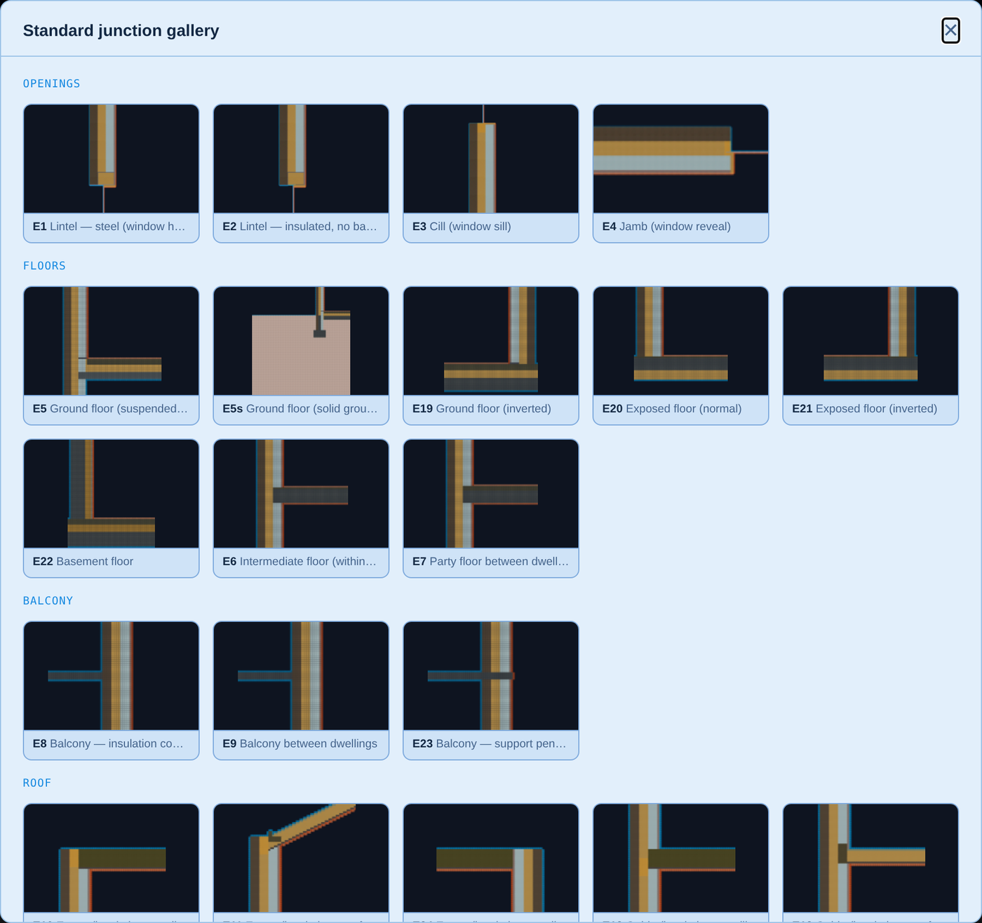
The library covers the full SAP 10 set: E1–E25 (lintels, cills, jambs, ground floors, balconies, eaves, gables, flat roofs, corners), the party-wall P-series (P1–P8) and roof windows R1–R4. Each loads with sensible accredited-reference build-ups, one-metre flanking arms, and every surface pre-assigned — a complete, ready-to-solve model.
Make it your build-up
Once a junction is selected, its construction appears as editable layer lists — one list per element (wall, deck, floor…), each labelled with its direction so you always know which end is outside. A live preview redraws as you edit, with the warm side tinted orange and the cold side blue, and a live Ψ figure re-solves after each change — you can watch the number respond to your design decisions before anything touches the canvas.
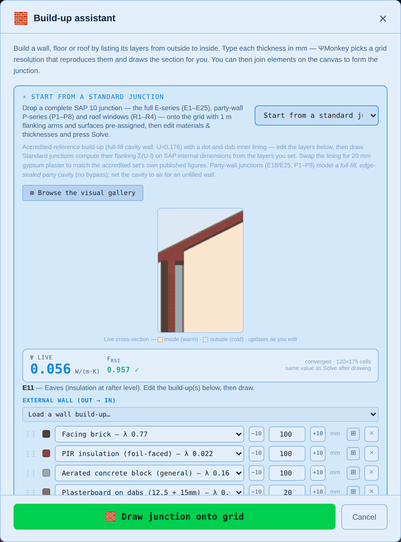
Start from a wall preset
Above the wall layers there's a build-up preset picker. Cavity masonry (full or partial fill) is the accredited default, and below it sit the constructions that are tedious to type out: timber frame brick-clad, with a service void, or with insulated sheathing; render and rainscreen; twin-stud / closed panel with 300 mm cellulose; and CLT with external woodfibre. Each arrives with its bridging fractions already set — 15% for studs at 600 mm centres once you count openings, headers and sole plates, 9% for a battened service void, 8% for twin-stud webs.
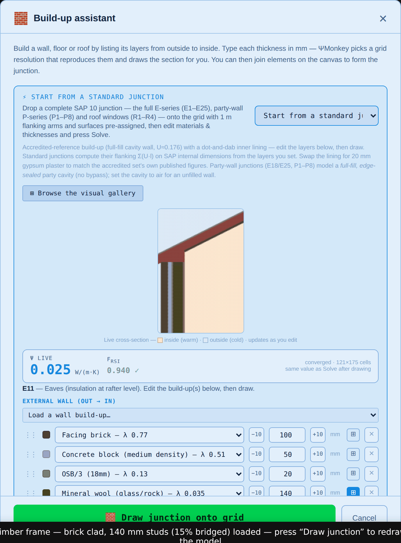
Picking a framed wall also changes the junction, not just the numbers. A masonry opening is closed with a proprietary insulated cavity closer; a timber-frame one is closed with a solid cripple stud, and the window has no closer to lap onto. At the eaves, a framed wall has no cavity to fire-stop and instead carries a solid header plate across the top of the studs, with the rafters running over it. ΨMonkey reads this from your build-up — any layer bridged by a timber means a framed wall — and draws the right detail without being told.
Editing layers
Each row is one layer: a material picker and a thickness in mm. The picker has a search box plus ★ favourites and 🕘 recents, and around 80 built-in UK materials with sourced conductivities. Thicknesses can be typed directly, stepped by 1 mm with the input's own arrows, or stepped by 10 mm with the −10/+10 buttons (or Shift+↑/↓ in the box). Add, remove and drag-reorder layers freely.
Bridged layers — studs, joists and battens
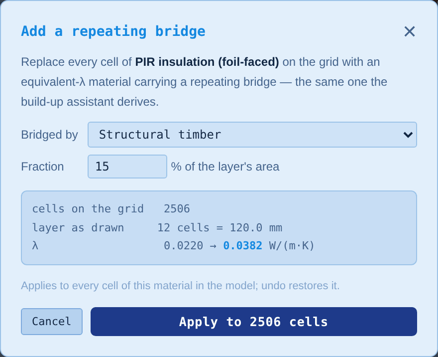
Real layers are often not homogeneous: insulation crossed by timber studs, a joist zone that is mostly air, a service void with battens. Click the ⊞ button on any layer to declare a repeating bridge: choose the bridging material and its percentage (50 mm joists at 400 mm centres = 12.5%). ΨMonkey computes the equivalent conductivity and uses it consistently in the drawing, the solver and the flanking calculation. You can do the same to a material you've already painted on the grid — see Editing on the canvas.
Draw, solve, and read the results
Press 🧱 Draw junction onto grid and the assistant stamps the whole model onto the canvas — construction, air regions, and every boundary condition. Then press ▶ Solve (top right). A few hundred milliseconds later you have your answer.
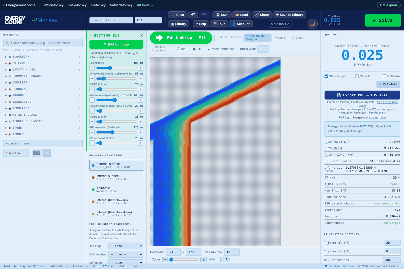
The two numbers that matter
| Result | What it means | What you want |
|---|---|---|
| Ψ (W/m·K) | The extra heat loss along the junction, per metre — the number that goes into the SAP calculation. | Lower than the SAP default for that junction type (the results panel spells this out for you). |
| fRsi | Surface temperature factor — how warm the coldest internal surface stays. Below the critical value, condensation and mould become a risk. | ≥ 0.75 for dwellings. The tool shows a ✓ or a warning. |
Trusting the number
The results panel isn't just the headline figure — it shows the full working: total heat flow, the 1-D flanking losses being subtracted (Σ U·l on SAP internal dimensions), the heat balance error, the ISO 10211 extent check and whether the solver converged. Green ticks all the way down means the model is numerically sound. There's also a ✓ Validate button that runs the solver against a suite of 21 published analytical and standard test cases — press it any time you want to see the engine prove itself.
Where the flanking came from
Ψ is a subtraction — the 2-D heat flow minus the 1-D losses the flat elements would have had anyway — so the number being subtracted matters as much as the model. The results panel names which basis was used, and the report carries it as a quality check:
| Flanking basis | When you get it |
|---|---|
| Convention Σ(U·l), internal dimensions | The model came from the assistant, so ΨMonkey knows the junction and its build-ups and subtracts exactly what a reference modeller would. This is the one you want. |
| Manual U·l | You entered your own flanking U-values and lengths — the certified route for thin-feature details. |
| Geometric auto scan — approximate | A hand-drawn or hand-edited model, where the tool has to find the flanking paths by scanning the drawing. Fine for exploring; not what you certify from. |
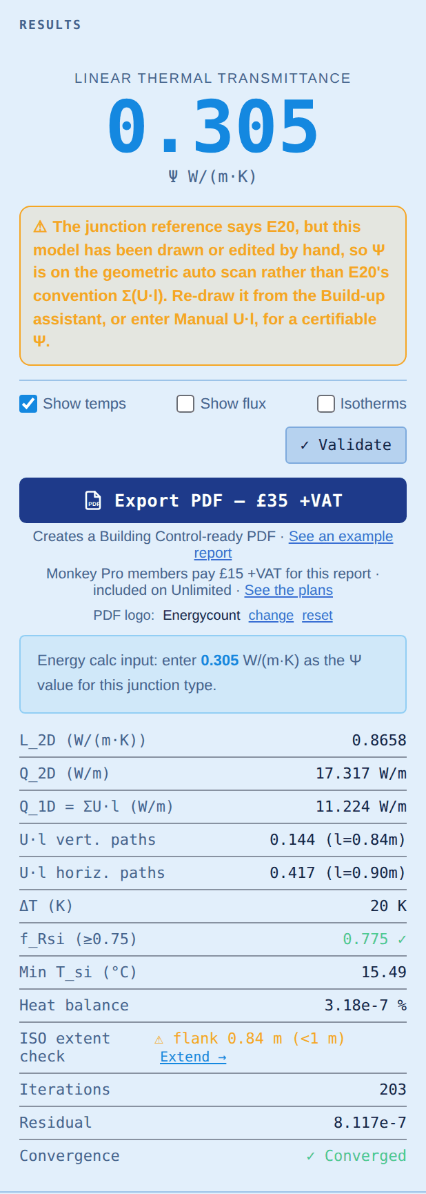
You'll see that amber note in a few other situations too: a project file saved by an older version that didn't record its build-ups, a layer too thin to draw on that junction's grid, or a fixed-resistance material (an air cavity) painted more than one cell thick. Each one is a case where the drawing and the arithmetic could quietly disagree, so the tool says it out loud rather than printing a confident number.
Editing on the canvas
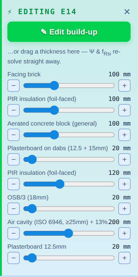
Once a junction is drawn, the Editing panel on the left keeps a slider for every layer. Drag a slider and the model redraws and re-solves as you watch — the fastest way to answer "what if the insulation were 20 mm thicker?" The − and + buttons at each end nudge by exactly 1 mm for precise tweaks, and ✎ Edit build-up takes you back to the assistant with everything preserved.
Drag a boundary
The sliders move whole layers of the build-up. When you want to move one interface — thicken the insulation at the cavity's expense, drop the sheathing back a few millimetres — pick the ↔ Move boundary tool and hover where two materials meet. The cursor turns into a resize arrow, the interface highlights, and the status bar reads out both thicknesses. Drag perpendicular to it and one material grows exactly as much as the other shrinks.
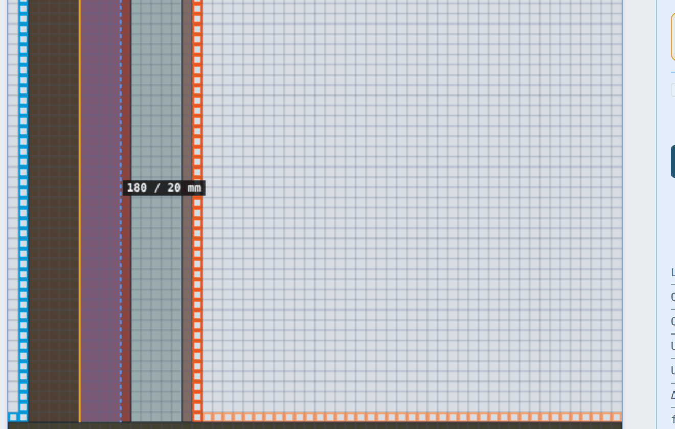
Two things make this safe. It only moves the stretch where those two materials meet, so dragging a wall/insulation interface doesn't disturb the same pair somewhere else in the drawing. And the travel is clamped to the layer being pushed: drag hard at a 50 mm cavity and it stops at 50 mm rather than quietly starting on the blockwork behind it. Because both sides move together, you can't open a gap — and a gap is not cosmetic here, since an unpainted cell is outside the model.
Add bridging to what you've drawn
Realised afterwards that a layer has studs in it? Any material that's actually in the model carries a ⊞ in the palette. Click it, pick the bridging material and fraction, and every cell of that material is replaced with the equivalent-λ version — the same derived material the assistant uses, so the solver, the U-value and the flanking all stay in step. Bridged materials show a ⊟ to take it back off again.
Handy canvas controls: mouse-wheel over the canvas zooms at the pointer (up to 800%), middle-button drag pans, + − 0 zoom from the keyboard, and the Fit button reframes the whole model. Zooming matters more than you'd think — some junctions (ground floors especially) model several metres of soil, so the interesting detail is a small part of the drawing.
Drawing your own detail
Two routes when your junction isn't in the library:
1. Build elements from layers, join them on the canvas
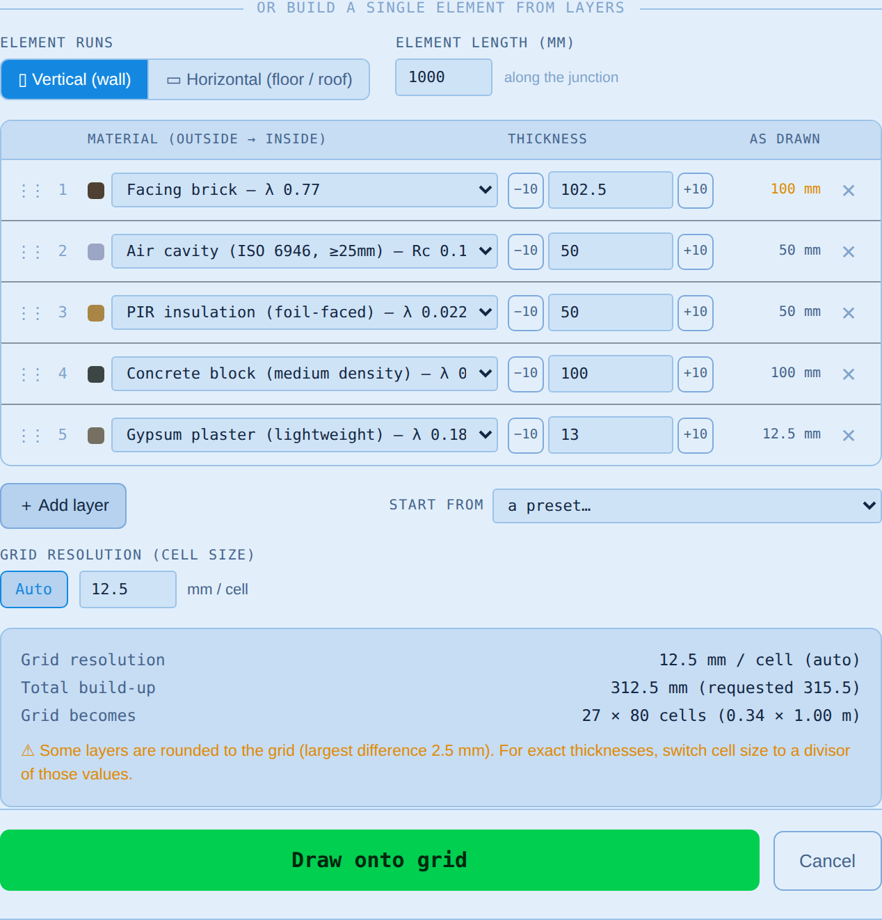
The lower half of the Build-up assistant builds a single element — a wall, floor or roof — from a layer list, exactly like the junction editor. Choose vertical or horizontal, set the length, and stamp it; ΨMonkey picks a cell size that reproduces your thicknesses and adds the surface boundary conditions. Stamp two elements so they meet, tidy the intersection with the paint tools, and you have a custom junction.
2. Paint it cell by cell
The canvas is ultimately a grid you can paint: pick a material, choose a tool (paint, line, fill, rectangular marquee) and draw the section directly — then tune it with the boundary drag and the ⊞ bridging control. Three rules keep a hand-drawn model honest:
| Rule | Why |
|---|---|
| Empty cells are outside the model. No heat flows through them — they behave as adiabatic cut-offs. | So the top and bottom of your flanking arms need no special treatment: just stop painting. |
| Paint boundary conditions on the empty cells just outside each surface — a line of External along the outer face, Internal along the room face. | BC cells are environment (air) nodes. Painted on top of material, they replace it — your wall silently gets thinner. The tool warns if you do this. |
| Keep every construction run continuous to the canvas edge it belongs to. | A gap lets "inside" and "outside" meet round the end of the wall, which wrecks the result. The edge dropdowns can also assign a condition to a whole edge in one go. |
Getting the number into SAP
The results panel tells you, in one line, exactly what to enter: the Ψ-value for that junction type in the SAP software's junction schedule (the y-value / thermal-bridging page). Give your assessor the value and the junction reference; they enter it as a calculated value in place of the default.
When the calculated value needs evidence behind it — Building Control ask, or the assessor wants it on file — Export PDF produces a report with the drawing, the temperature field, the build-up schedule with every conductivity and its source, the full ISO bookkeeping, fRsi, the validation status and a verification reference. It's £25 +VAT per report, one junction per report; the calculator itself, and everything above, is free without sign-up.
Good habits & common pitfalls
| Habit | Why it pays |
|---|---|
| Start from the standard junction, even for unusual details. | You inherit correct geometry, seeds, boundary conditions and flanking conventions, then adapt — far safer than building from a blank grid. |
| Change one thing at a time and watch the live Ψ. | You learn which layer actually drives the result — usually the insulation continuity at the joint, not the thicknesses. |
| Check fRsi as well as Ψ. | A junction can have an acceptable Ψ and still fail the mould check. Both print on the report. |
| Compare against the SAP default before celebrating or panicking. | Defaults vary widely by junction (0.05 to 1.0+). The results panel names the relevant comparison. |
| Save your project (💾) and use the Library. | A saved .json reloads exactly, so a junction can be revisited when the spec changes — and the Share button gives colleagues a link. |
If a result looks wrong
Read the amber notes first — under the Ψ figure and in the results panel. They cover the things that most often make a number wrong rather than merely surprising: the flanking basis, a layer too thin for the grid, a fixed-resistance material painted too thick.
Then zoom out and look at the whole drawing. Nine times out of ten a surprising Ψ is geometry: a construction run stopping short of the canvas edge, boundary-condition cells painted onto material (they're flagged with a diagonal cross), or inside and outside air meeting around the end of an element. The assistant-drawn junctions get all of this right automatically — hand-edits are where to look. And be suspicious of a result that looks too good: a Ψ well below the published value for that junction type usually means something has been subtracted that shouldn't have been, not that you've designed something remarkable.
Quick answers
Do I need to be a thermal modeller to use this?
No. The assistant route — pick junction, edit layers, solve — needs no modelling knowledge at all. The conventions (surface resistances, flanking subtraction, internal dimensions) are applied for you and printed transparently in the results panel.
How accurate is it?
The solver passes a 21-case validation suite (analytical solutions and standard test cases) which you can run yourself with the ✓ Validate button, and the standard junctions reproduce accredited reference constructions to within the tolerance you'd expect of a 2-D screening model. Every result carries its own convergence and heat-balance audit.
Why is my Ψ-value negative?
Sometimes it should be. SAP measures on internal dimensions, and at inverted corners and re-entrant junctions that convention over-counts the flat-area losses, so the junction "gives back" a little. Everywhere else, a negative Ψ almost always means the flanking subtraction has over-counted — which is why the tool shows it in amber and points you at the flanking basis rather than congratulating you.
It says Ψ is "on the geometric auto scan" — what does that mean?
That the model has been drawn or edited by hand, so ΨMonkey can't use the standard junction's flanking convention and has to find the 1-D paths by scanning the drawing instead. It's a reasonable approximation for exploring, and poor at thin features like openings. For a figure you'll certify, re-draw the junction from the assistant (which restores the convention) or enter Manual U·l with your own flanking U-values.
Does it handle timber frame?
Yes. Load a timber-frame wall preset in the assistant — the stud zone comes with its bridging fraction already set — and the junctions adapt to it: an opening gets a solid cripple stud instead of a masonry cavity closer, and an eaves gets a header plate across the studs with the rafters running over it. You can also add bridging to a layer you've already painted, with the ⊞ control in the material palette.
Can I model a junction that isn't in the library?
Yes — start from the nearest standard junction and edit it, stamp elements with the single-element builder and join them, or paint freely on the grid. See Drawing your own detail.
What does the paid report add?
Nothing changes in the calculation — the £25 +VAT PDF is the evidence pack: drawing, temperature field, sourced material schedule, ISO checks, fRsi, and a verification reference Building Control can check. The calculator itself is free.
Is my model saved anywhere?
Your work autosaves in your browser and can be exported as a .json project file (💾 Save). Nothing is uploaded — models stay on your machine unless you share or export them.